
Part -7 – Excel SUM MAX MIN AVERAGE
Download Excel Templates – Excel SUM MAX MIN AVERAGE
Excel SUM MAX MIN AVERAGE (without solution)
Excel SUM MAX MIN AVERAGE (with solution)Note:Become an MS Excel Expert
Learn how to organise, format and calculate data smoothly. Develop skills to master excel tools, formulae and function. Analyze data from different perspectives.
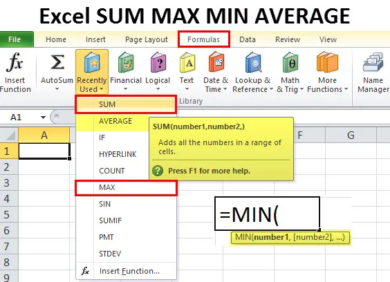
Transcript For The Video – Excel SUM MAX MIN AVERAGE
Having looked at some of the basic calculations in terms of multiplication, let us try to use some formulas to add some levels; here, let us write the total salary we would also like to calculate, say, the maximum salary of our employees. The minimum salary is drawn and, let’s say, the average salary. So we would like to calculate all these for monthly as well as annual. So for doing that, let’s start with the monthly and go immediately below column F, which is F23. There are two ways of doing this one: there is an excel menu that determines how the functions are. So if you have to total this function, what you need to use is a sum. SUM. And for this, we can look at how do we insert functions. So let’s click here we go to, we can choose a different kind of functions. Let’s choose SUM because that’s what we want to do. We want to sum the total the monthly salary and let’s press ok. And once we have done that, you need to click here and choose the numbers or the range which you want to sum total. This can be done by dragging from the top till the bottom of the employee table. So this will sum total the monthly salary of the employees, and what you will do next is just press ok, and you will find that the formula which is equal to sum F4 colon F21 is being executed. And the sum total comes out to be 92700 USD as the monthly salary of XYZ company. Now, this was the 1st approach. The 2nd approach would be to let me delete the original formula 1st. It would be typing the formula, which means you type equal to your need to type sum total SUM open bracket and here it defines the numbers. The number 1, number 2, within this bracket, you can choose the full range from F4 till F20 and don’t press enter as of now. Close the parentheses 1st and then press enter. With this, you will find that you have created your 1st set of formulas which is the sum total of this monthly salary. Now, this is how you can proceed normally when you are using excel a lot may be the 2nd approach is much more suitable because you well versed with the formulas; the 1st approach involves the uses of a mouse, which becomes a bit tedious at times. So I would highly recommend that you must use the 2nd approach. Now let us try to find the annual salary of the total employees. Now here I will teach you another set of approach, so let us look at the home and the many here, which is an auto sum. Just click on this auto sum, and you may find that your full formula, which is equal to sum G4 till G22, is being shown in the cell. The next thing you will have to do is just to press enter, and you will find the overall annual package or annual salary has been calculated using this formula. So as you may have seen, you know excel being an intelligent tool; it automatically identifies what you are trying to do based on your previous history, and sometimes it really works well. So I would like to recommend that if you have used such kind of formulas, please do a double check on whether this formula is totally accurate. Now let us move to the next set of formulas, and the approach will essentially remain the same. The 1st approach would be to insert this function from the top and find the relevant formulas. So here we want to find the maximum salary. So the formula would be MAX bracket open and the selection of numbers. So I have selected this function MAX, and I will press OK and in order to choose the numbers, I will have to click here and select the range. So this approach will be as simple as this, I will just press OK, and what we find is the maximum salary is 9200 dollars. Let us try to calculate the maximum salary, which is the annual salary using the 2nd approach for the annual one. So this would be as we do for others we use equal to this is basically excel way of telling that anything that comes after equal would be a formula. So this is equal to and use max with a bracket open what would this mean is you need to now select this range of numbers, and let us select the full range in term of annual salary, and we close the bracket and press enter in order to find the maximum salary. So this is the maximum monthly salary, and we have the annual salary calculated using the formulas. So let us now calculate the minimum salary as well this will be equal to the formula for a minimum is MIN, this is the formula this returns the smallest number in a set of value, and it ignores logical values and text. So open brackets, select the range within which you want to find the minimum and close the bracket. So what we find the minimum salary is 2100 dollars. Likewise, let’s quickly find the minimum for the annual salaries. MIN bracket open and lets quickly select the range and bracket closed. So this is 25200 dollar is the minimum salary. What about the average salary, there are 18 employees, and each employee is drawing a different kind of salaries. So what will be the average salary? So it is very easy if you are using excel, and again you just need to know the function. As intuitive as it can be, the average is the formula that we will use, and the format remains again the same. Let us select the range from F4 to F21 and bracket close. So that we find is the average salary is 5150 USD. And let us find the average again for the annual salary this is bracket close, which is 61800 dollars. So as you may have seen, we have written these formulas twice, one in this set of a column which is F and the same formula was written in this column, which is G. Now, there is essentially a shortcut by which you can totally avoid writing a formula in the G column if you have written that formula for the F column. Say, for example, let’s take the case of total salary, which is the monthly salary. Now for this, we have already written the formula which consists of this block. Ok, and we just need to shift this block from F to G block. For calculating the total salary. So the way we can do it is earlier we had learned copy and paste from Microsoft word to excel sheet. Here what we will be doing is copy and paste from MS Excel to MS Excel itself. So this means copying the formula from column F to column G. So what we will do is we will select the cell just right click go to copy and select the cell G. I will do the right click again. Select cell G right-clicks and paste. We find that the formula gets copied from left to right, the difference being that since we have shifted one column here the column, the sum total for the column also gets shifted. So this is the way in which you can actually copy and paste your set of formulas. A regular tip for shortcuts CTRL C and CTRL V. This is copied, and this is paste. Now let me show you what this shortcut tip is all about. Let me delete the annual salary again. Go back to the monthly salary; what I need to do is just use the keyboard buttons and press CTRL and C the moment I do that, it gets highlighted, this means that copy has been activated; the next function that I need to do is paste. So, where do I need to paste this formula? I want to paste this formula into cell G23. How will I do that? This is CTRL and V., So the moment I type CTRL and V, you will find that the formula gets replicated in cell G. So this is how you know you can work along with the shortcut tip on copy and paste.
Recommended courses